Lab 9
The purpose of this lab is to map out a static room by collecting ToF data at various coordinates within a preset layout in the lab.
Control
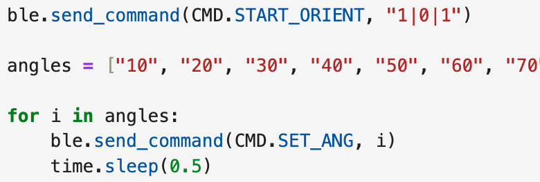
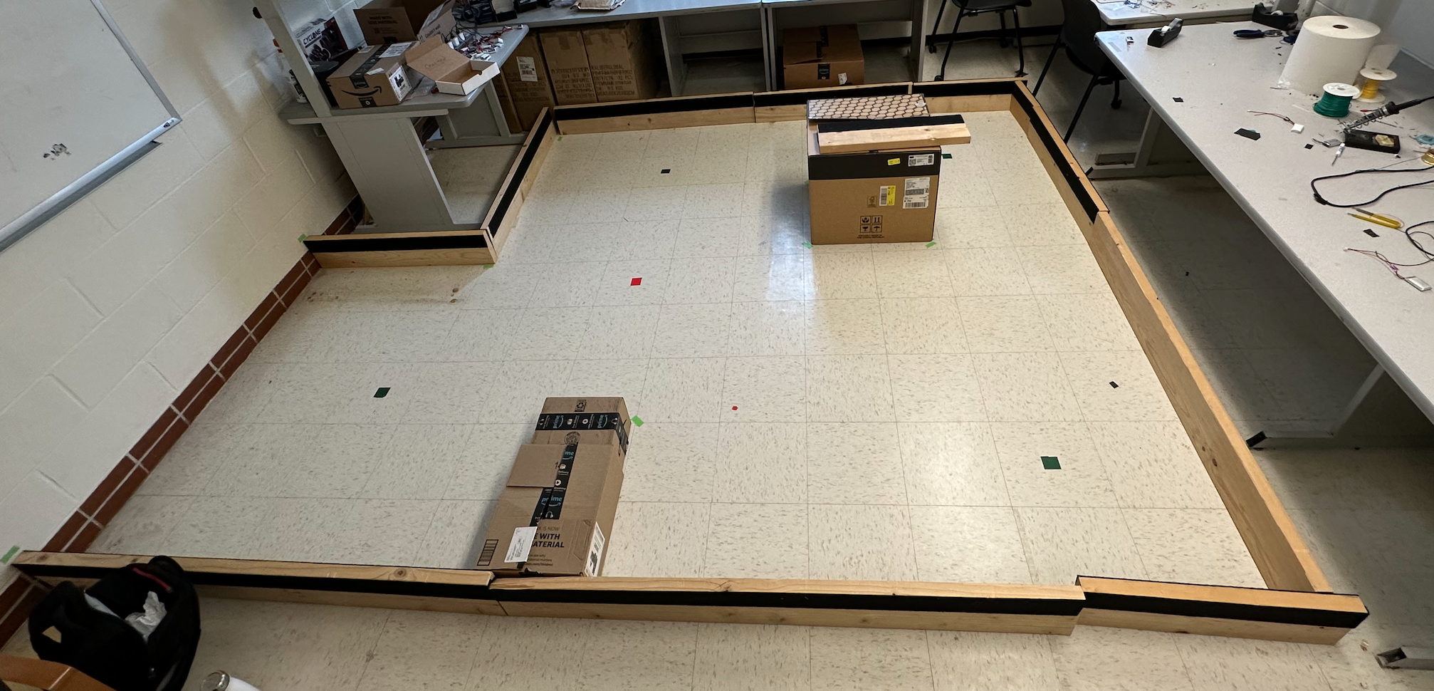
In order to collect ToF data at each coordinate, the robot needs to do on-axis turns in small increments. This is accomplished by repurposing the orientation PID controller from Lab 6. In addition to the original PID controller case that I wrote for the previous labs, I implemented a new case that allows me to redeclare the desired angle for my PID controller. Then, I could run a for loop in Jupyter that would send a command every 0.5 seconds, giving the robot time to settle at each angle then turn to the next desired angle. I chose to use a step of 10 degrees in order to capture as much data as possible while also ensure the step was large enough for the PID to actually move the robot (based on the gain values). The robot started at 0 degrees yaw for each trial and took 36 steps until it completed a full 360 degree on-axis rotation. The process was repeated for each of the four coordinates in the lab map. A photo of the lab map is also shown below.
Below is a short video that demonstrates the robots ability to spin on-axis and collect data at the various coordinate locations. The ToF data is being collected using the main while loop, and then the final array is sent via Bluetooth once the movement is finished.
Mapping Results
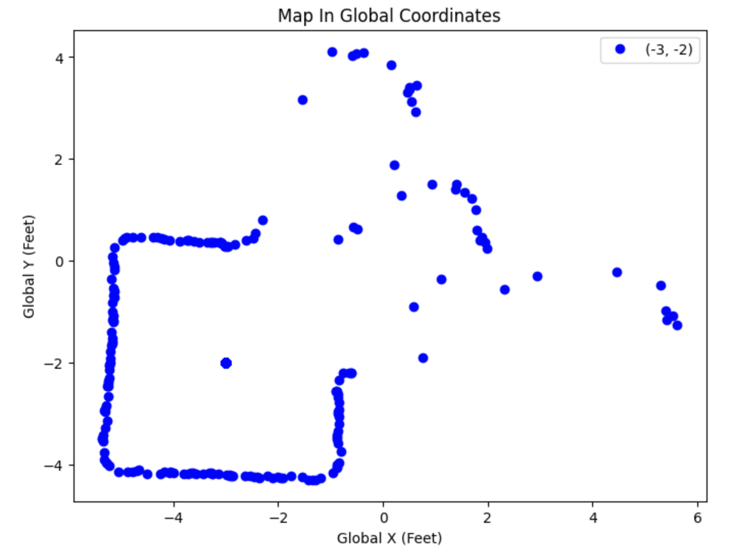
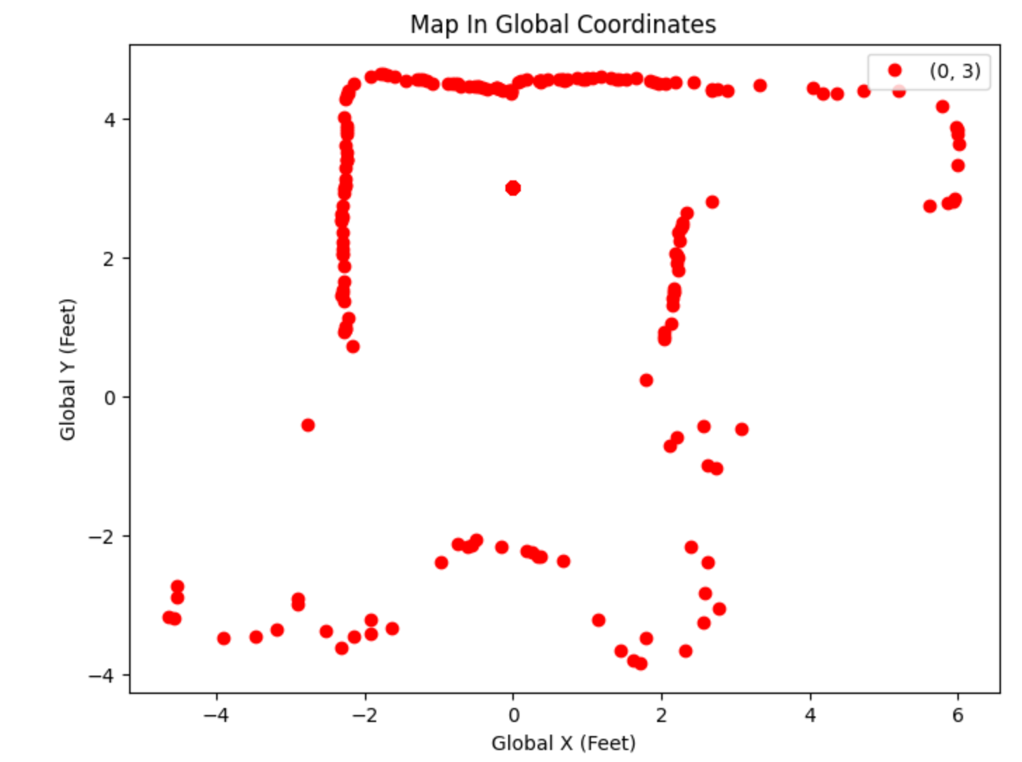
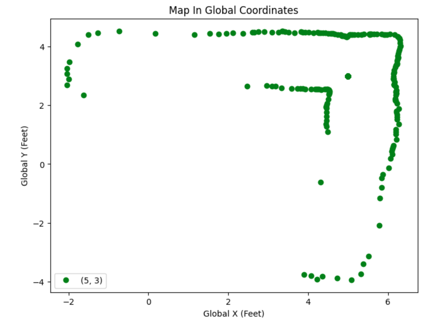
After placing the robot at each of the four coordinates within the lab map (marked by the pieces of tape in the photo above), I then plotted each of the scans using polar coordinates. Because we know the yaw value (angle) and the radius (ToF reading), we can map out the surroundings in (X,Y) global coordinates for better visual comprehension. Below are each of the scans after their conversion to the global cartesian coordinate system. Each tile on the floor represents one foot, and each scan is labeled in the legend as its local origin of the scan.
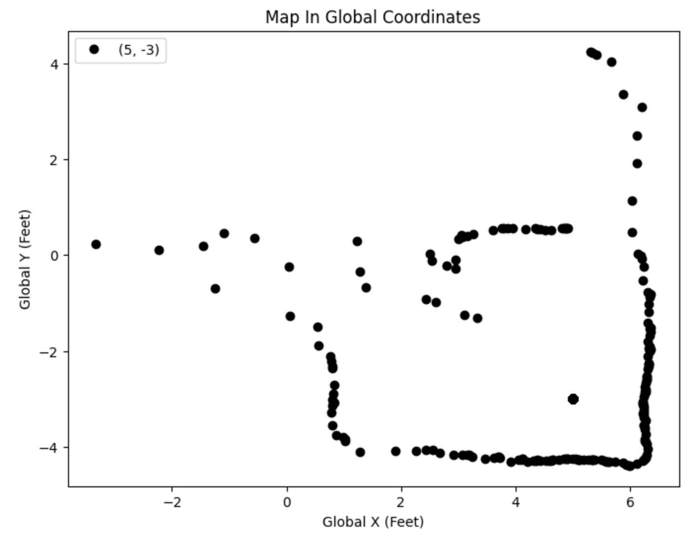
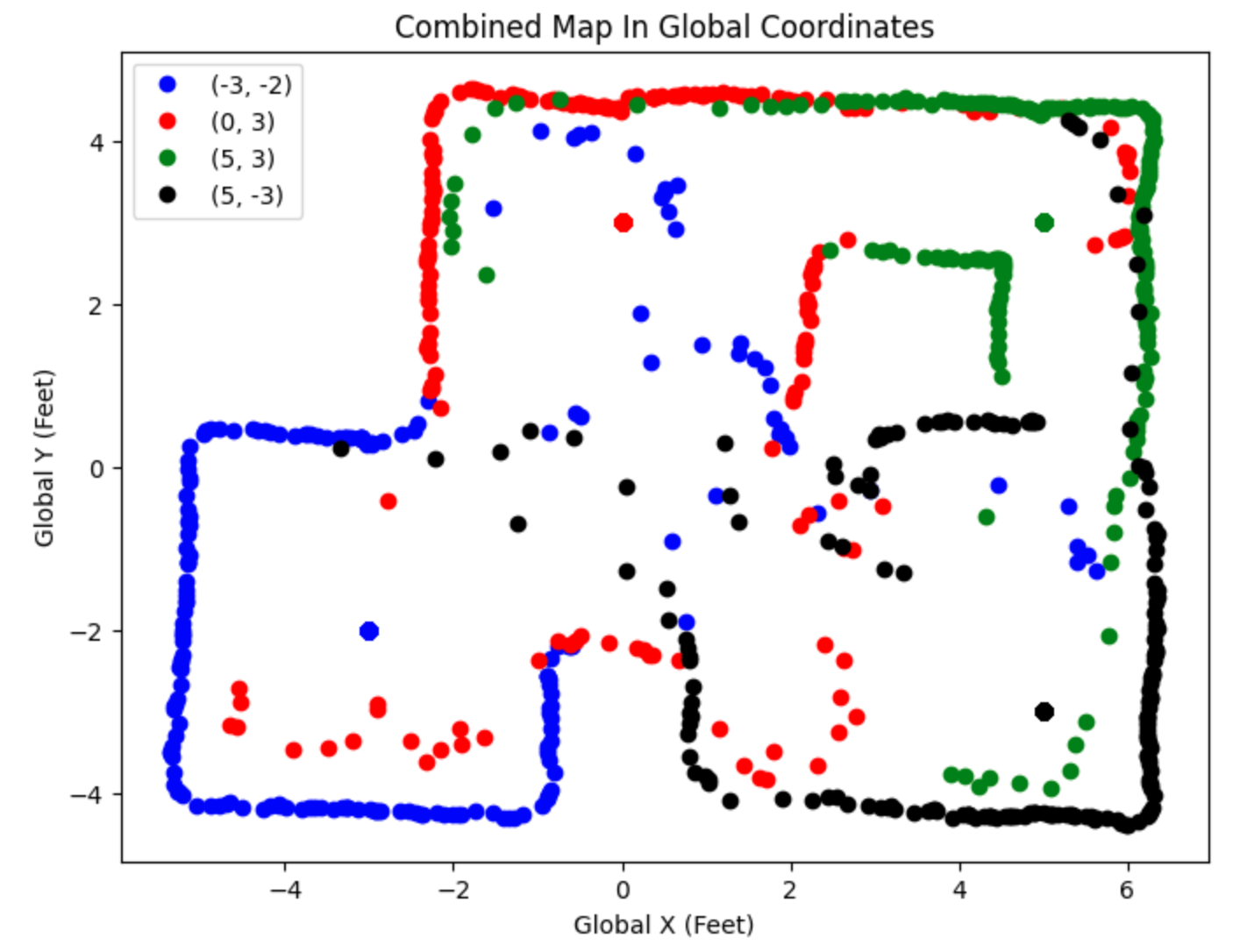
After collecting each of the individual scans, the final step was to save each to a CSV file and combine them into an aggregate plot. This plot would hopefully show the full map with barriers and obstacles in their correct global position. This plot is shown below.
Line-Based Map
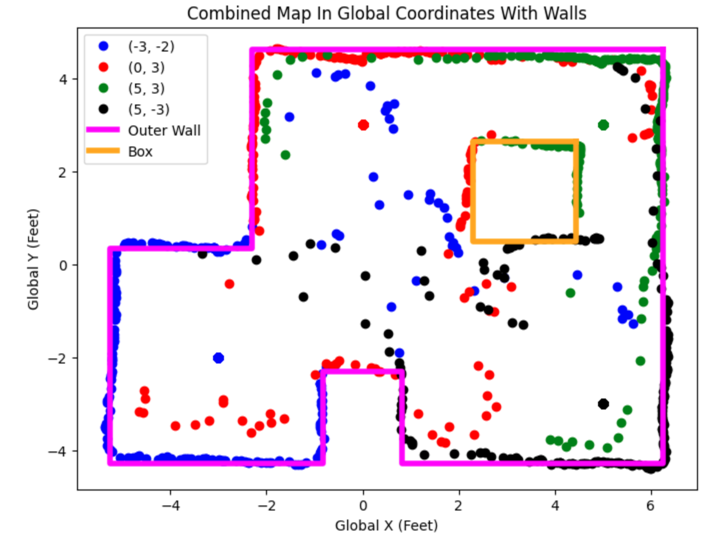
Using the completed map above, the final step is to estimate the walls and obstacles using a line-based map. This is done by visually ignoring the extraneous data points and trying to estimate the walls and obstacles in the map. Then, by manually plotting lines to fit the general trend of the map, I was able to complete the final mapping task. The final map is shown below.
Lab 9 Takeaways
This was a really valuable lab as we started to get more into the localization aspect of this course. By utilizing multiple sensors and techniques developed in previous labs, the robot is able to accomplish more complex tasks and have a more developed and robust system. I ran into some trouble with collecting accurate ToF data, and after hours of debugging, it ended up being an issue with whether my IMU was face up or face down. I plan to look further into this issue to hopefully avoid similar problems in the last few labs. Overall, this was a very fun lab, and it was very rewarding to see an accurate scan of the lab map.