Lab 2
The purpose of this lab is to connect the IMU to the Artemis and study the behavior of the onboard accelerometer and gyroscope. In the process, we will design a complementary low pass filter to gain more accurate readings from the two sensors. Additionally, we will test out the RC car to understand its tendencies, speeds, and maneuverability.
Prelab
The Prelab consisted of reading the IMU datasheet and becoming familiar with the functionality of the breakout board.
Task 1: Set up the IMU
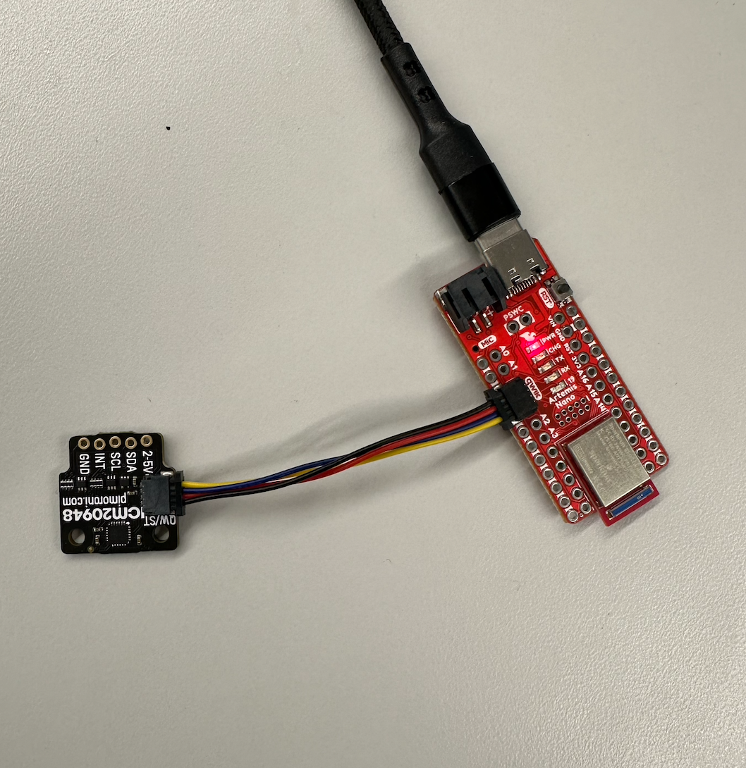
The IMU uses a QWIIC connector to connect to the Artemis board. A picture of the cable and proper connection is shown below. Once the IMU was hooked up, we could run the "Basics" example from the Arduino Library. This was the first exposure to the onboard accelerometer and gyroscope. Before beginning, we had to change the AD0_VAL value from 1 to 0. This changes the final bit of the I2C Address, and thus changes whether or not the data is being sent or received. For our purpose, we will set it to 0.
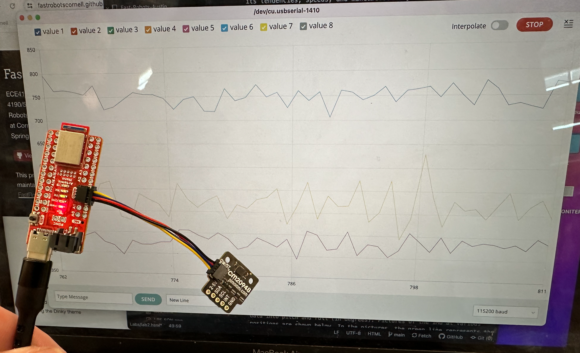
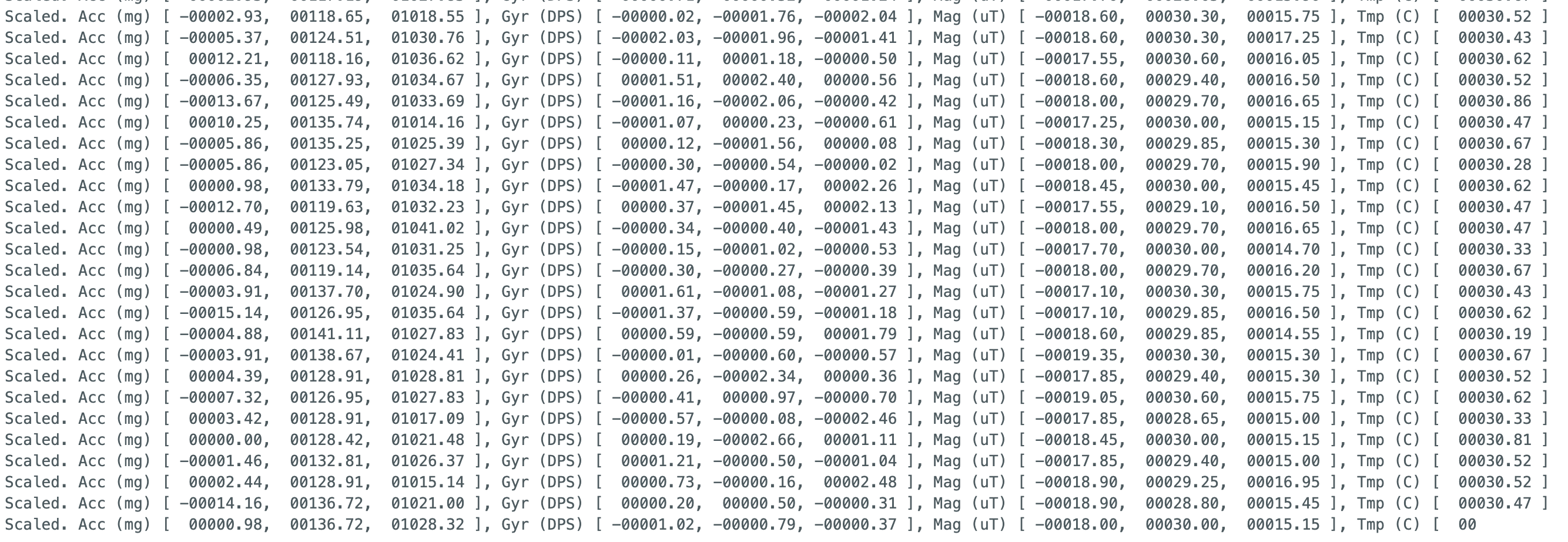
A few pictures of the "Basics" example running are shown below. The first picture is a snapshot from the Serial Plotter on the Arduino IDE with the IMU present in the photo as well. The second photo is the continuous stream of data points in the Serial Moniter of the Arduino IDE. Both of these confirm that the example is working and the IMU is hooked up properly.
Task 2: Accelerometer
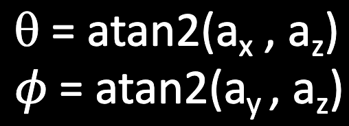
The next task was to focus on the accelerometer. To start, we implemented the equations provided in lecture using atan2 to convert the accelerometer data into pitch and roll (in degrees). Pictures of the IMU at various positions are shown below. In the pictures, the green line represents the pitch and the blue line represents the roll. In order to capture each of these graphs, the IMU was help against the side of the table or flat on the table to ensure it was held as close to 90 degrees as possible.
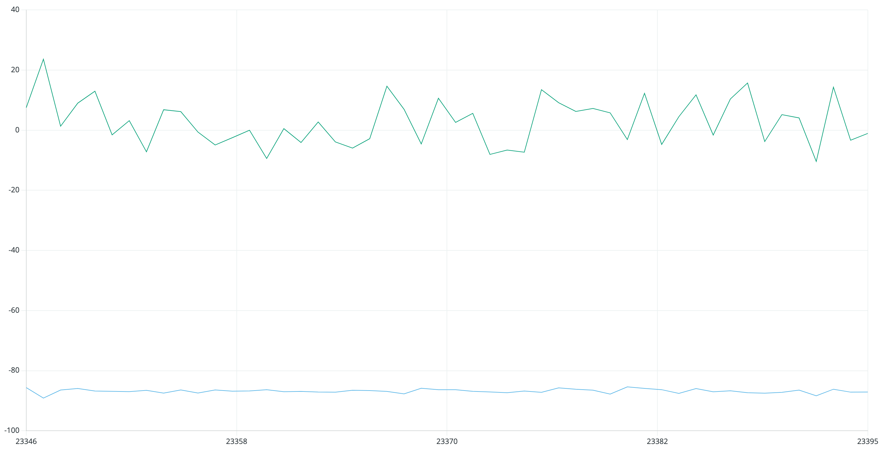
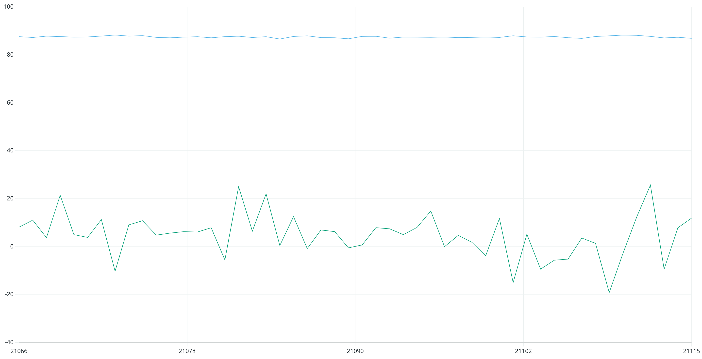
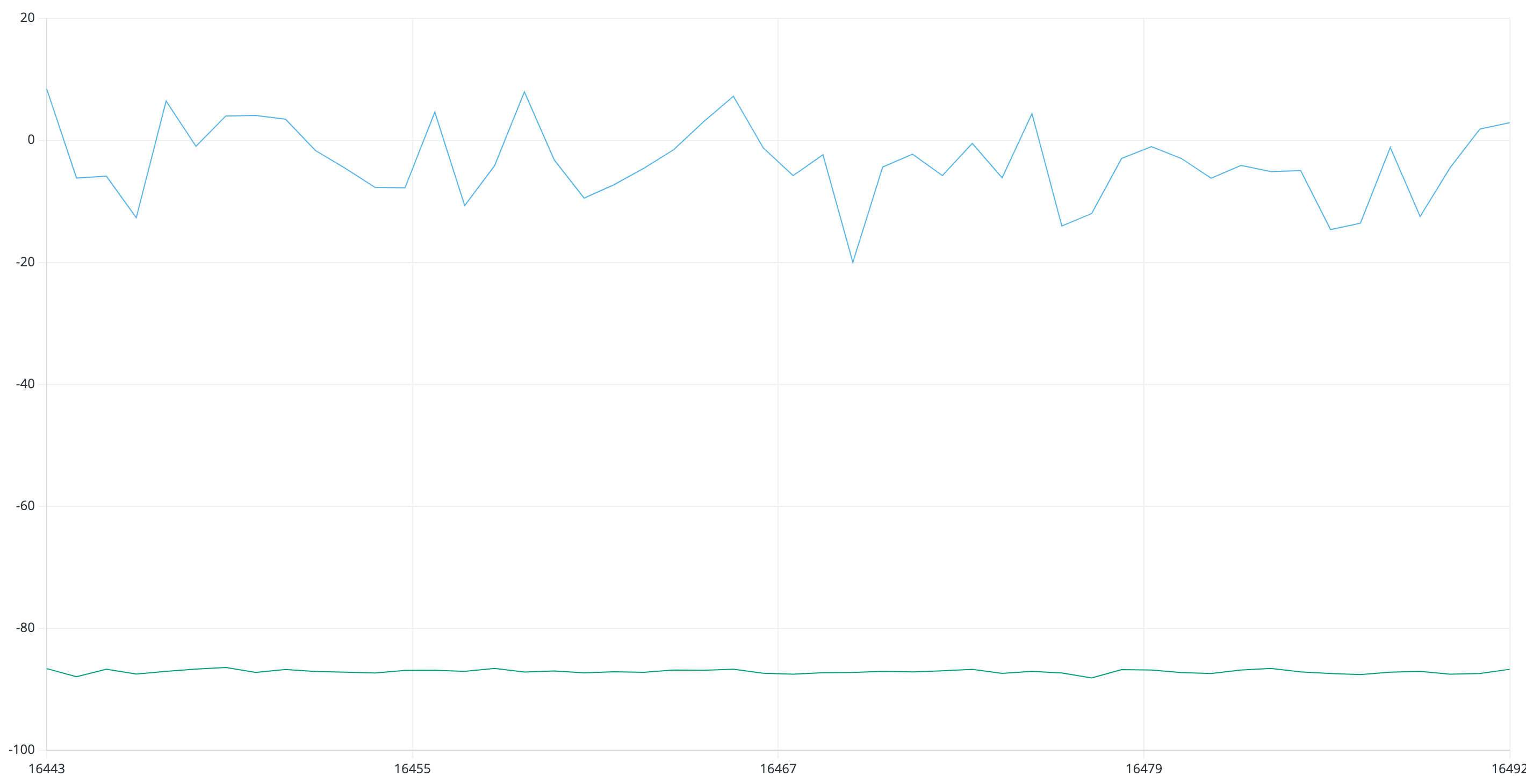
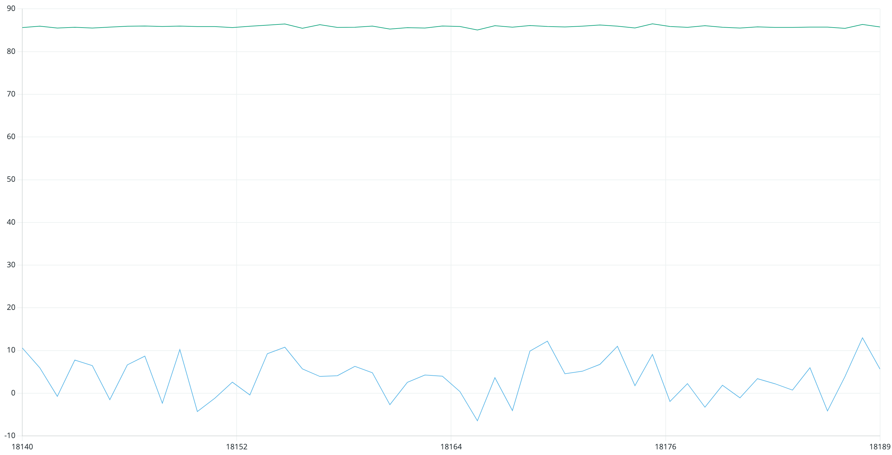
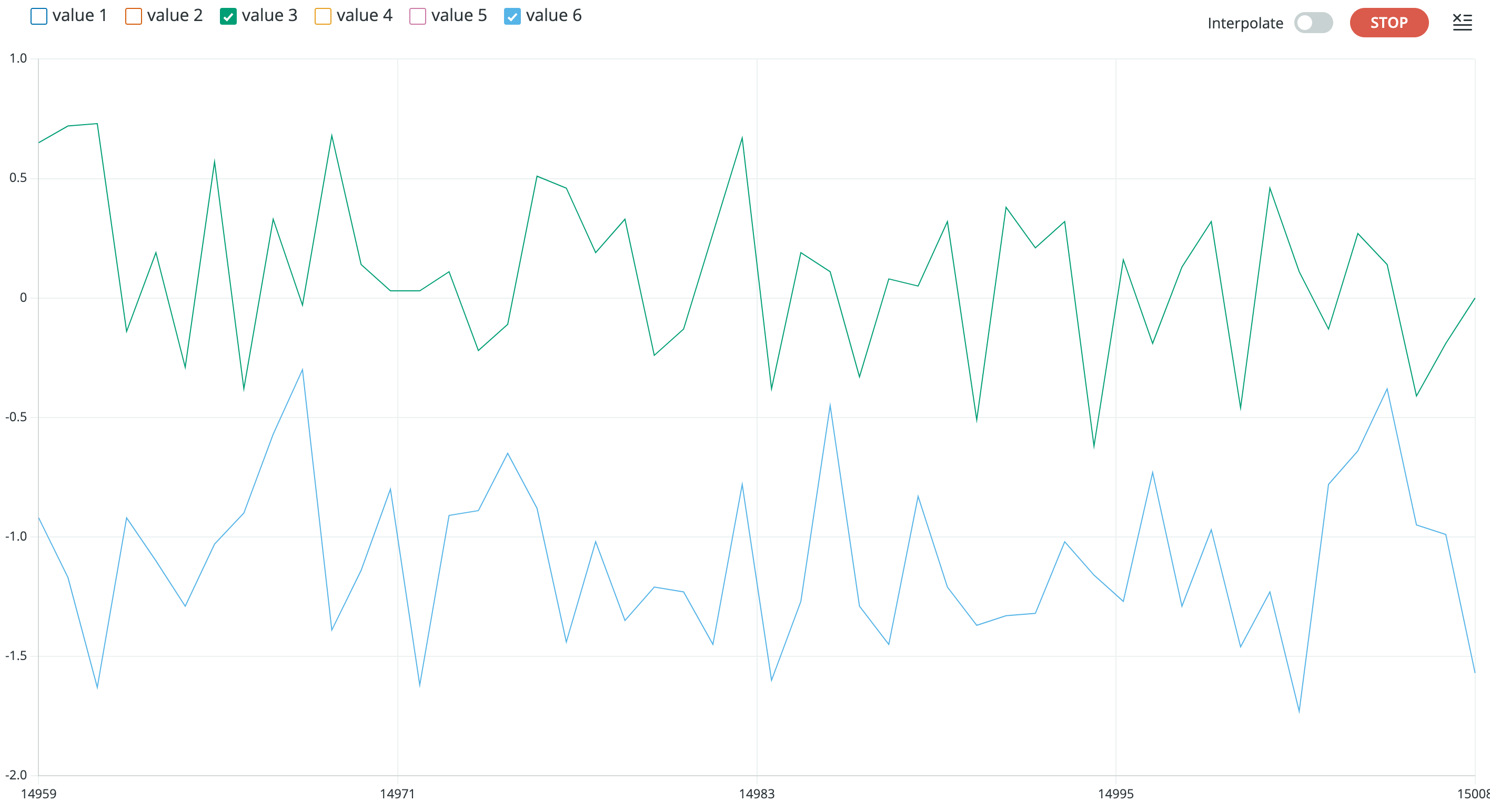
Like any sensor, there is bound to be some sort of offset that requires calibration to fix. For my IMU, I found that the accelerometer was roughly 3 degrees off. While this does not seem like a large amount, it can cause issues for my car down the road, so I will multiply the values by a correction factor to account for this offset.
Task 3: Fourier Transform
In order to analyze the amount of noise affecting the accelerometer, we want to create a Fourier Transform to convert the data into the frequency spectrum. This was done using a simple Fourier Transform off the internet, and a picture of the accerometer data in the frequency spectrum is shown below. The associated graph in the time domain is also shown for reference.
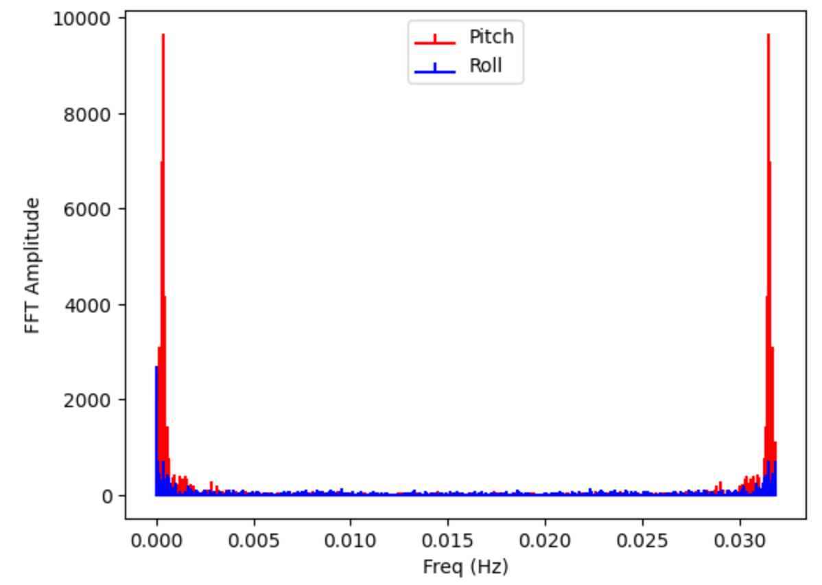
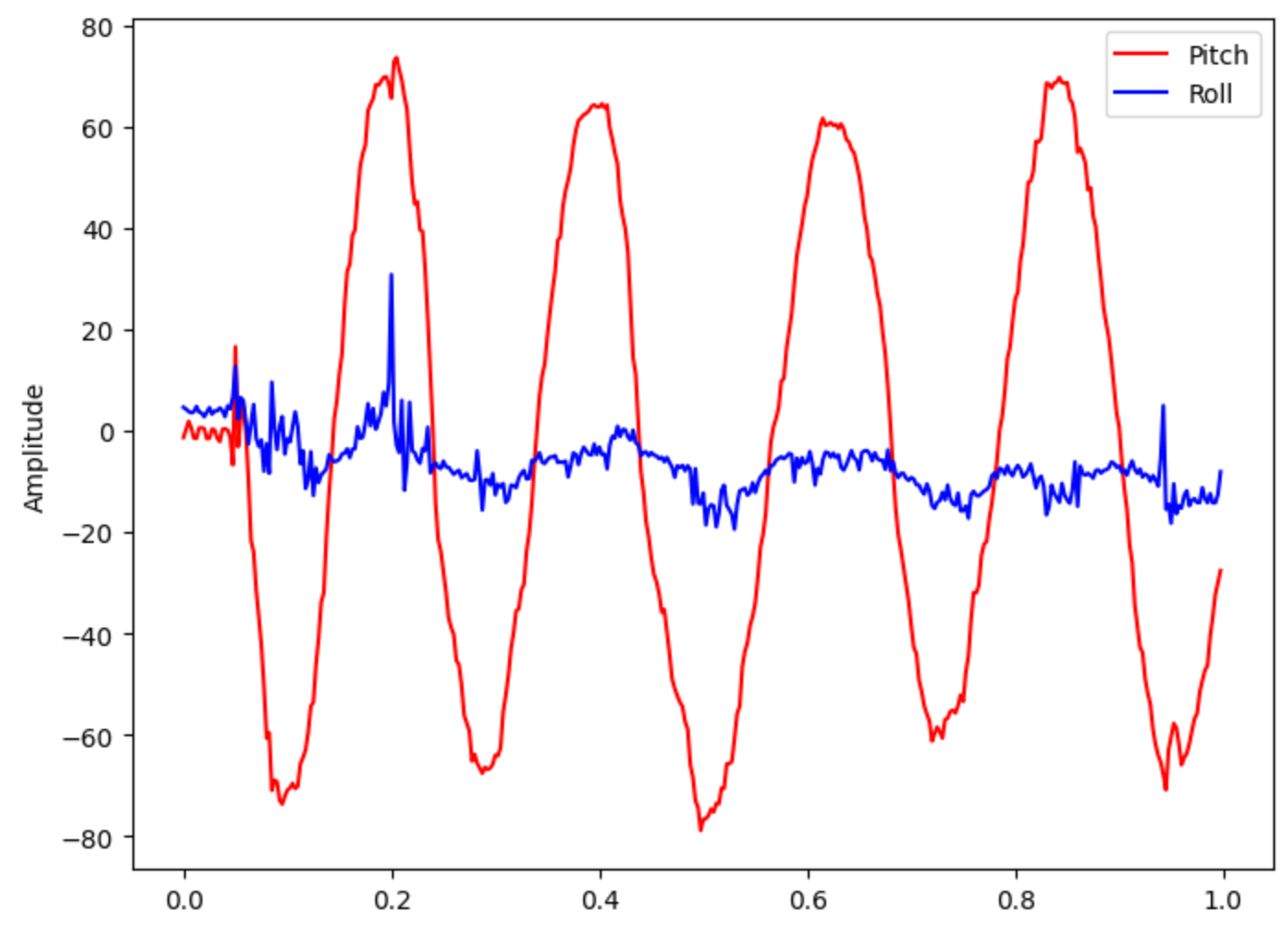
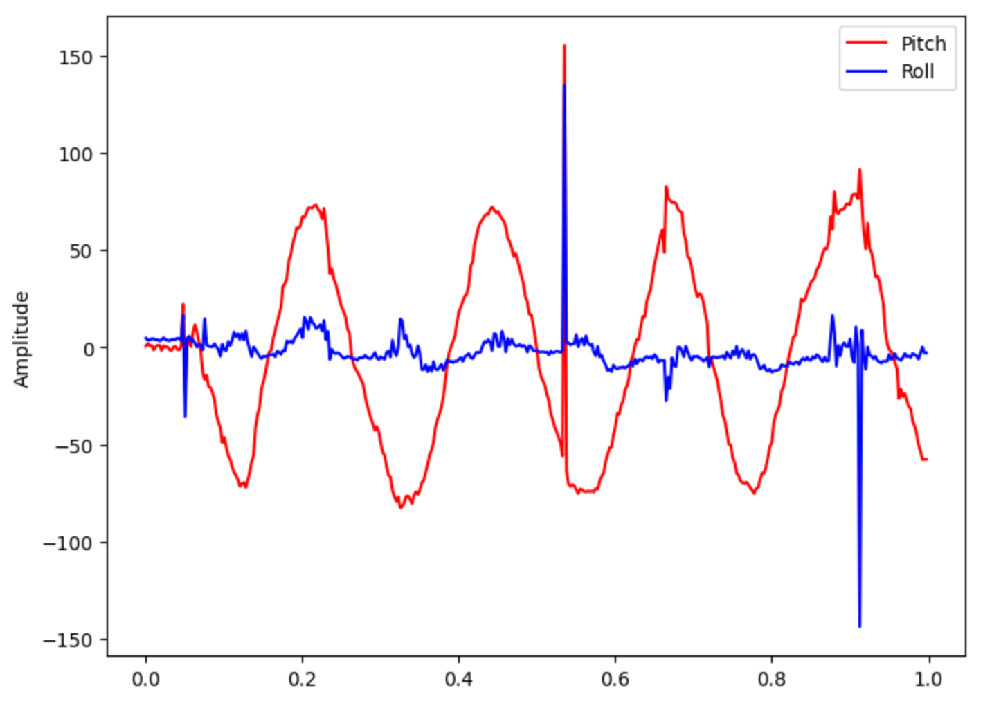
After analyzing the results, a low pass filter was implemented to help reduce the noise at high frequencies. Although there is a built-in filter on the IMU already, this is good practice to implement our own LPF. The equation for the LPF that was implemented is shown below and is from the slides from lecture. The data was then plotted again but this time filtered through the LPF. A picture of the plot is shown below as well. While it is not the exact same data as above, you can tell that the peaks are smoother, and there are less random spikes in the data.

Task 3: Gyroscope
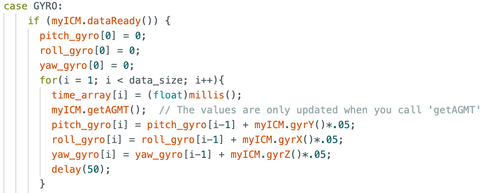
The next task was the analyze the gyroscope functionality. First, just like the acceleromater, we needed to convert the data into pitch, roll, and yaw (in degrees). Since the gyroscope outputs data in deg/s, we can multiply the output by a "dt" value using consecutive timestamps and then add to the initial gyroscope reading in order to get current angle in degrees. A snippet of my case from the Artemis is shown below to illustrate this math.
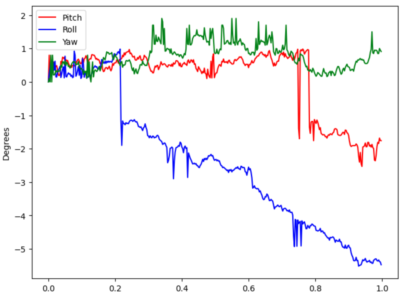
When plotting the pitch, roll, and yaw from the gyroscope, I first looked at the data when the IMU was sitting flat on the table. The graph of this data is shown below. As you can see, there is significant drift in the data points. This is due to the "dt" multiplied term. It causes the output to "run" away from the resting 0 point.
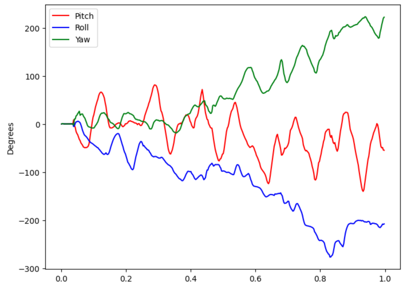
This trend is mimicked when the IMU is moved through space. A plot is shown below where I moved the IMU randomly and rotated it in several ways. You can see that the drift is especially noticeable in the roll and yaw directions, yet it can be seen in all three measurements. This is drastically different from the acceleromater data which always returned to the 0 position when the ICM was placed back down on a flat surface.
Task 4: Complementary Filter
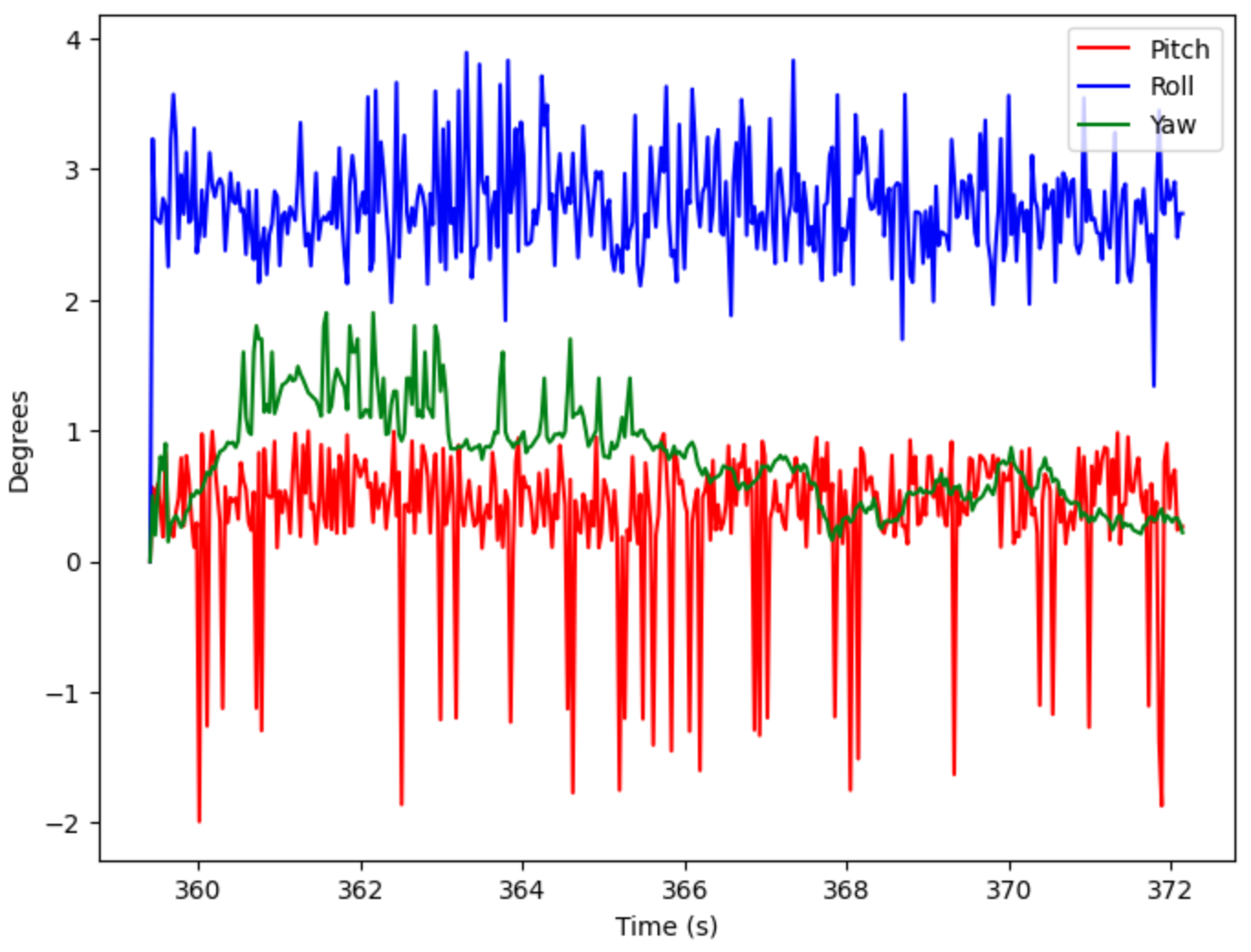
To fix the issue of the gyroscope data drifting away from the 0 position, we can implement a complementary filter. This filter combines the data from the accelerometer and the gyroscope in order to create more accurate and stable angle outputs. The equation for the complementary filter was taken from the lecture slides and is shown below. I then tested the IMU flat on the table to test the drift as before. The plot of this test is shown below. The drift is basically gone, there is just a little noise in the sensor readings due to vibration and sensor noise.

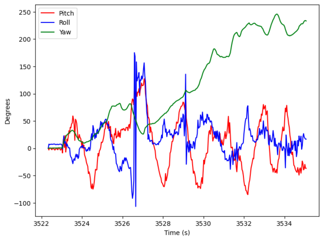
The complementary filter was tested again, but this time I moved the IMU in random rotations and tangential movements. The drift is almost entirely removed for pitch and roll, yet yaw still has some drift. This make sense because the accelerometer has no yaw measurement, so the filtered yaw value is just the gyroscope reading. A picture of the plot is shown below.
Task 5: Sample Data
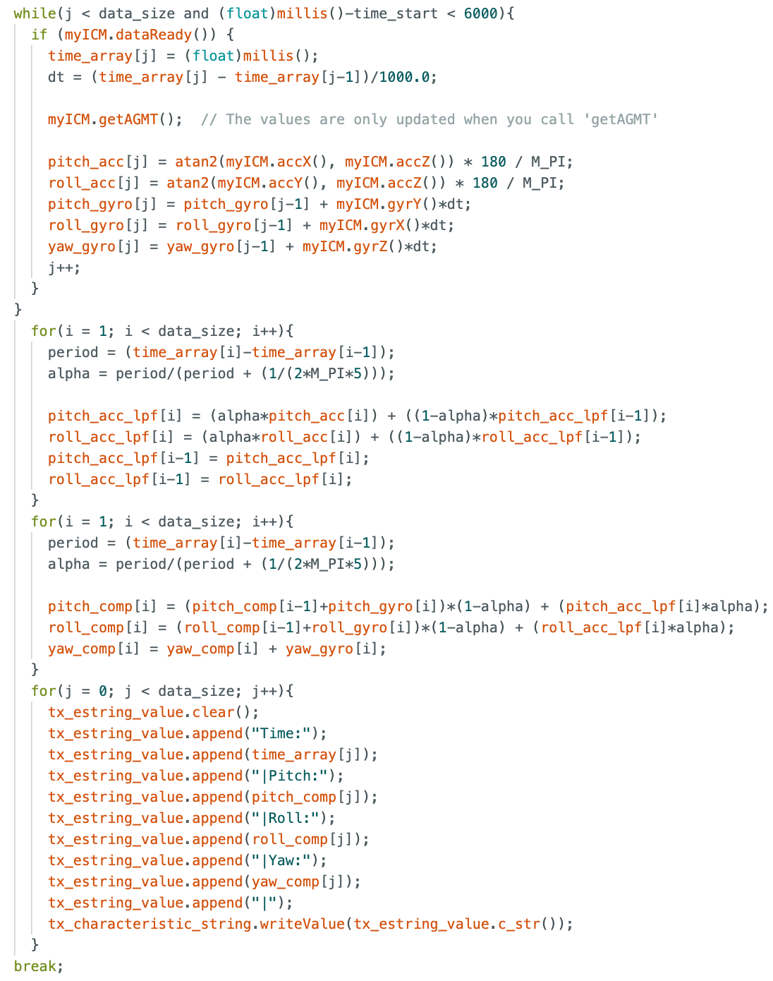
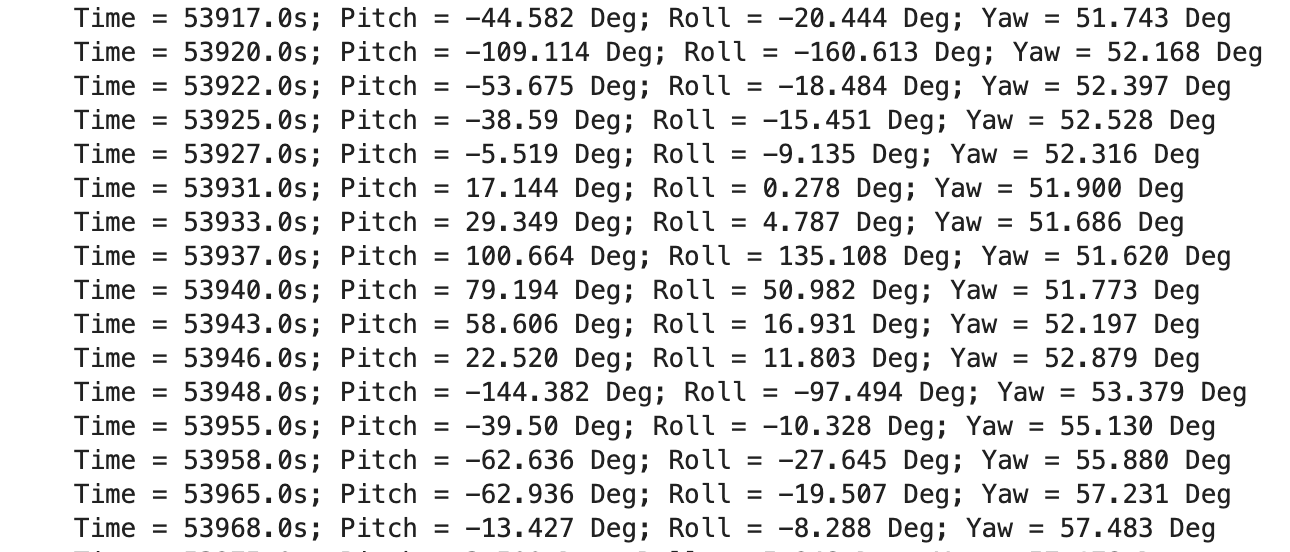
In this task, the goal is to speed up our sampling rate so we can collect data as quickly as possible. This is done by removing all delay statements, print statements, and adjusting the main loop so it no longer waits for the IMU to be ready before moving through the loop. Using this method, I was able to get a sampling rate of about 3.45 ms. My Artemis code and some of the print statements in Jupyter are shown below. Based on the print statements, we can see that the Artemis runs faster than the IMU can produce new values.
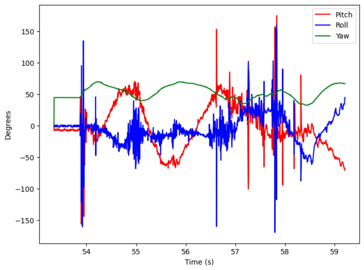
To show the capacity of how much data could be sent, I recorded for over 5 seconds. A plot of this data is shown below with a time axis to illustrate the data.
Task 6: Record a Stunt
The final task of the lab is to play with the RC car and record a stunt. Below is a video of the RC car performing some basic functionality such as moving forward and backward, turning, and doing a flip. The video ends when the RC car ends up on its side. This will prove to be a potential issue moving forward as the robot must move autonomously.
Lab 2 Takeaways
This lab was both fun and very informative. The accelerometer and gyroscope were both very frustrating to work with in the beginning, yet I was eventually able to get the hang of them. They will both be very useful moving forward to track the RC car's position and orientation in space. Also, knwoing how to implement Fourier Transforms and low pass filters will be useful to analyze data in future labs. Finally, it was very nice to be able to play with the car and get a feel for what kind of functionality we will be able to implement later on in the semester.