Lab 7
The purpose of this lab is to implement a Kalman Filter to help speed up the behavior from Lab 5 (linear PID control).
Estimating Drag and Momentum
The first step in implementing the Kalman Filter is to build the state space model of our system. We need to estimate the drag and momentum terms for our A and B matrices. By using our ToF sensor data, we can measure the steady state speed of our RC car at a given step response. For my tests, I chose to use 50% of the maximum u(t) value. This means the PWM of each wheel will be half of its maximum of 255. It did not make sense to run my car at full speed, as I will rarely be running the car at that speed for the upcoming tasks as control will be more valuable than speed.
During my tests, I set the ToF sensor to long ranging mode. This will decrease the amount of accuracy, yet it will allow my the ToF sensor to start collecting accurate data further out than when it is in short mode. We need the extra distance to allow the car to ramp up to its steady state velocity. After running a few trials, I found that my steady state speed at 50% max speed is roughly 2300 mm/s. Using this speed, I found that the 90% rise time was roughly 1.25 s. Using these values, I can calculate the momentum and drag terms mentioned above. The equations to solve for these values are shown below. Substituting the correct values into these equations, I arrived at a drag value of 0.217 N, and a momentum value of 0.118 kg*m/s.


Initialize Kalman Filter
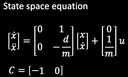
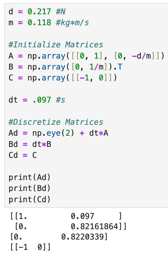
The A and B matrices are defined based on the equations shown below. The C matrix is simply [-1 0]. Additionally, a dt value is required to help discretize the matrices. This value was found to be 0.097, or 97 ms, based on the data collected in the trial mentioned above. Then, once initializing the state vectory for both x0 and P0, I chose values for the process noise and sensor noise. For Sigma_1 and Sigma_2, I used the equation presented in lecture and arrived at a value of 32.11 mm and 32.11 mm/s respectively. For Sigma_3, I started with a value of 20 mm as suggested in class.
Implement and Test The Kalman Filter
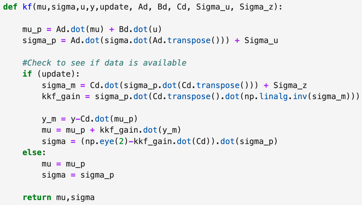
I then implemented the Kalman Filter into Jupyter using the function provided in the lab document. The function as well as my implementation of the Kalman Filter are shown below. I proceeded with the 5000 level task by making the Kalman Filter run faster than the TOF sensor collection frequency. This means that the Kalman Filter will interpolate and predict the TOF data based on previous values. These changes are already implemented in the code shown below.
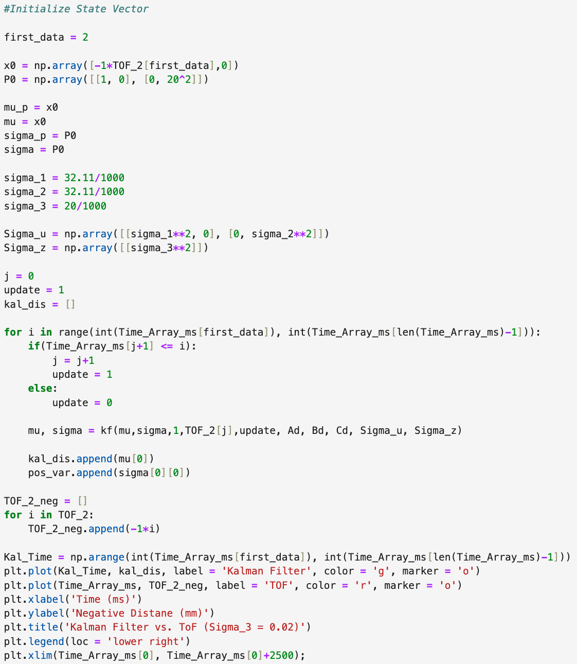
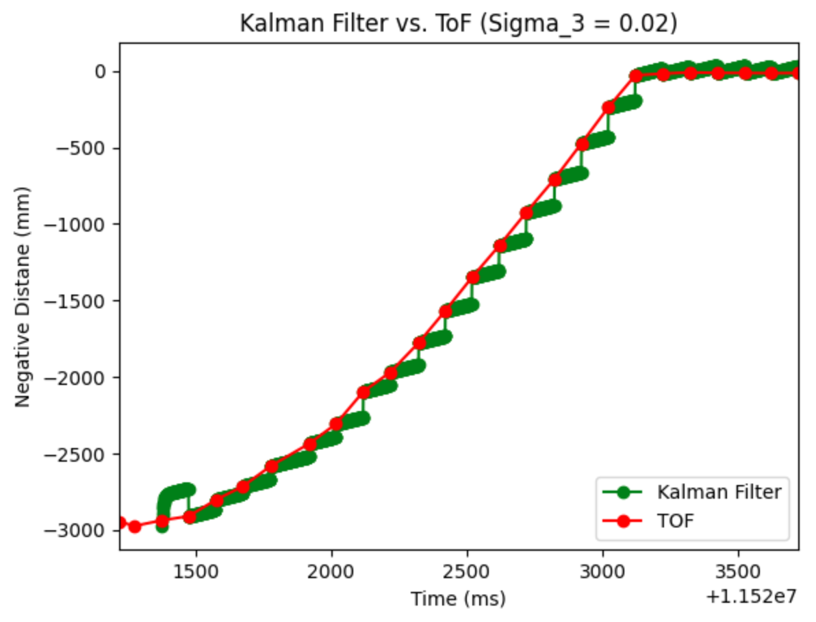
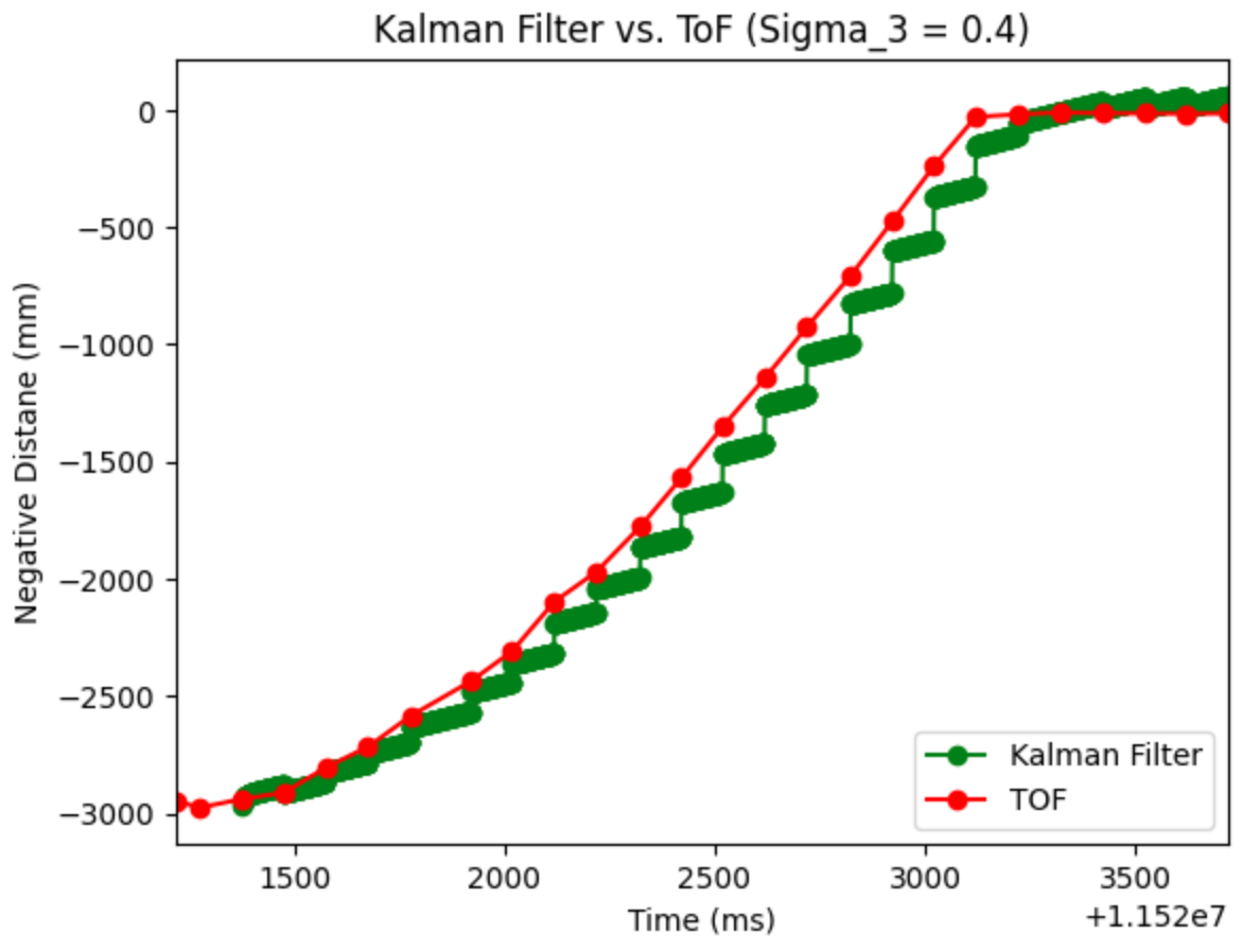
In order to test the Kalman Filter's sensitivity to sensor noise. By changing Sigma_3 from 20 to 400, I was able to see how the Kalman Filter would respond. In theory, the higher the value, the less the Kalman Filter will respond, and the smaller the noise, the Kalman Filter will be unable to work. The two plots are shown below.
Extra Credit
I have not implemented the Kalman Filter onto my RC car, but I hope to do so during Lab 8.
Lab 7 Takeaways
I can see how the Kalman Filter will help improve the speed of our robot moving forward. It is very useful to correct noise based on dynamics and current ToF sensor readings. I hope to implement it onto my car to help with control in the future.