Lab 12
The purpose of this final lab is to have the robot navigate through a set of waypoints in the environment as accurately as possible. This lab is intentionally open ended, so the method for completing the navigation procedure is up to the student.
Introduction
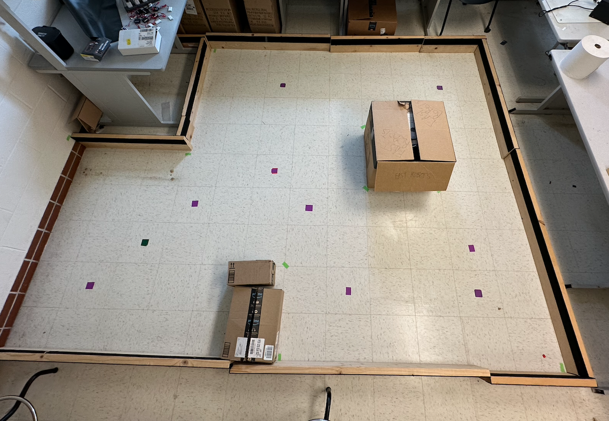
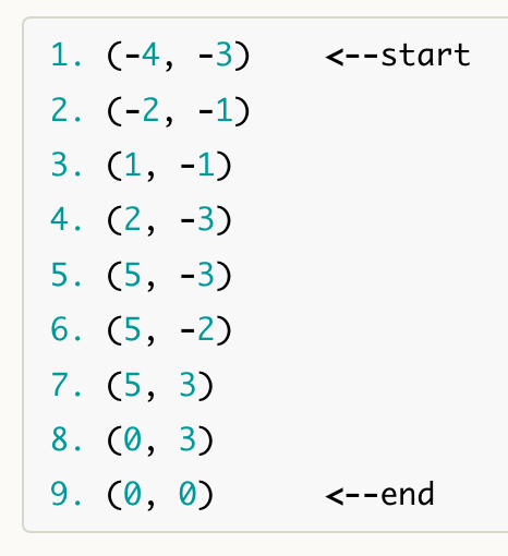
For this lab, the defined waypoints were given in the lab outline. These points, as seen in the figure below, are marked by purple tape within the lab map. I also included the numeric waypoints, where each tile on the floor of the lab is 1 foot (1 unit). As mentioned earlier, this lab is intentionally open ended. The various options that I attemped were localization, ToF & PID control, and hard coding.


Localization Procedure
For my first attmept, I wanted to try and build off of lab 11 and utilize localization and Bayes Filter to successfully naviagte the map. This was done by using the provided code from Lab 11 and altering it so that I could save the belief position and use it as the input for the next localization iteration. The thought process was then that the belief would be compared to the next defined waypoint, and the robot could adjust its orientation and distance values to move to the correct location.
Unfortunately, while my robot localized nearly perfect at the four corner positions described in Lab 11, my robot had difficulty localizing correctly for this lab. For each attempted trial, my robot would arrive at a belief, often 99% or higher, that it was at a location outside of the map or across the map. This made it very difficult to correclty implement any type of navigation plan as my robot would think it would have to cross the map to arrive at the correct position. I tried to correct for this by hard coding the first orientation and distance measurements, yet I ran in to this issue for nearly every point I attemped localization at.
ToF & PID Control
Given the time constraint of limited time with finals, I decided it would be best to try an alternative method rather than spend hours trying to debug my localization attempt. I thought the next best thing would be ToF control. This involves using the ToF data to measure the robot's current distance from a wall or obstacle, and moving forward a delta distance using linear PID control. The orientation and distance values were found using standard trig functions.
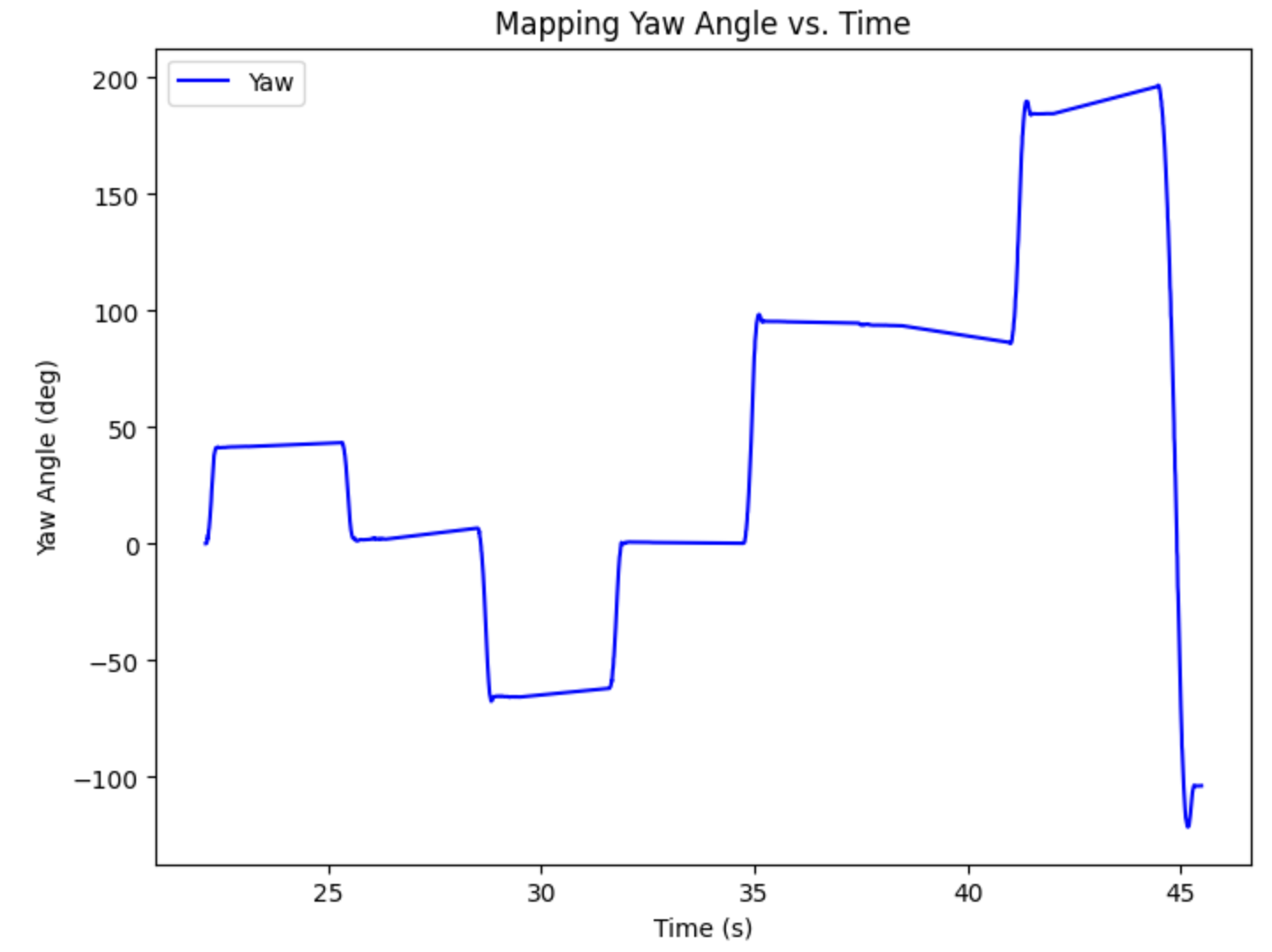
The orientation control was relatively straight forward to implement. I was able to accurately turn to the correct angles easily and quickly, which allowed me to focus more on the distance issues because I knew my angles were working correctly. A plot of the yaw over time is shown below.

In order to accomplish implementation of the ToF sensors, I defined a new case that would allow me to change the "desired distance from the wall" in real time from Jupyter. For example, if I wanted the robot to move forward 1 foot, and I know the current ToF reading is 3 feet, then I could simply change the desired distance to 3-1 feet or 2 feet. Once the robot settles within a set threshold of the desired distance, I could then conduct orientation control and rotate the robot so it is facing the next defined waypoint. A video of my most successful trial run is shown below.
As seen above, I had to add an additional waypoint between points 1 and 2 because the ToF sensor could not accurately sense the far distance at the 45 degree angle between points 1 and 2. Additionally, my robot only made it to point 6 out of the 9 before it began to stray off course, and I had to stop the trial. In hindsight, while I thought this was due to inaccurate linear PID control, it was most likely due to my robot not driving completely straight, causing the errors of my orientation control to compound. If I had more time with this lab, I would definitely work to make this method more successful.
Hard Coding
For my final attempts, I resorted to hard coding the navigation path using PID orientation control for the angles and timed, forward driving for the distances. I used trig to solve for the angles between each points, and then utilized PID orientation control developed in the previous labs to correctly orient in that direction. Then, I developed a new case that would just spin my wheels forward, driving it in a straight line. Starting this lab, I also ran into issues of my left motor not spinning as quickly as my right motor. In the previous 11 labs, my wheels have spun nearly perfectly in sync, eliminating the need for a correction factor. However, for this lab, I had to offset my wheels by a factor of 1.22. Once I was able to recallibrate my wheels, I was more successful in my trials. My (nearly) successful trial is shown below.
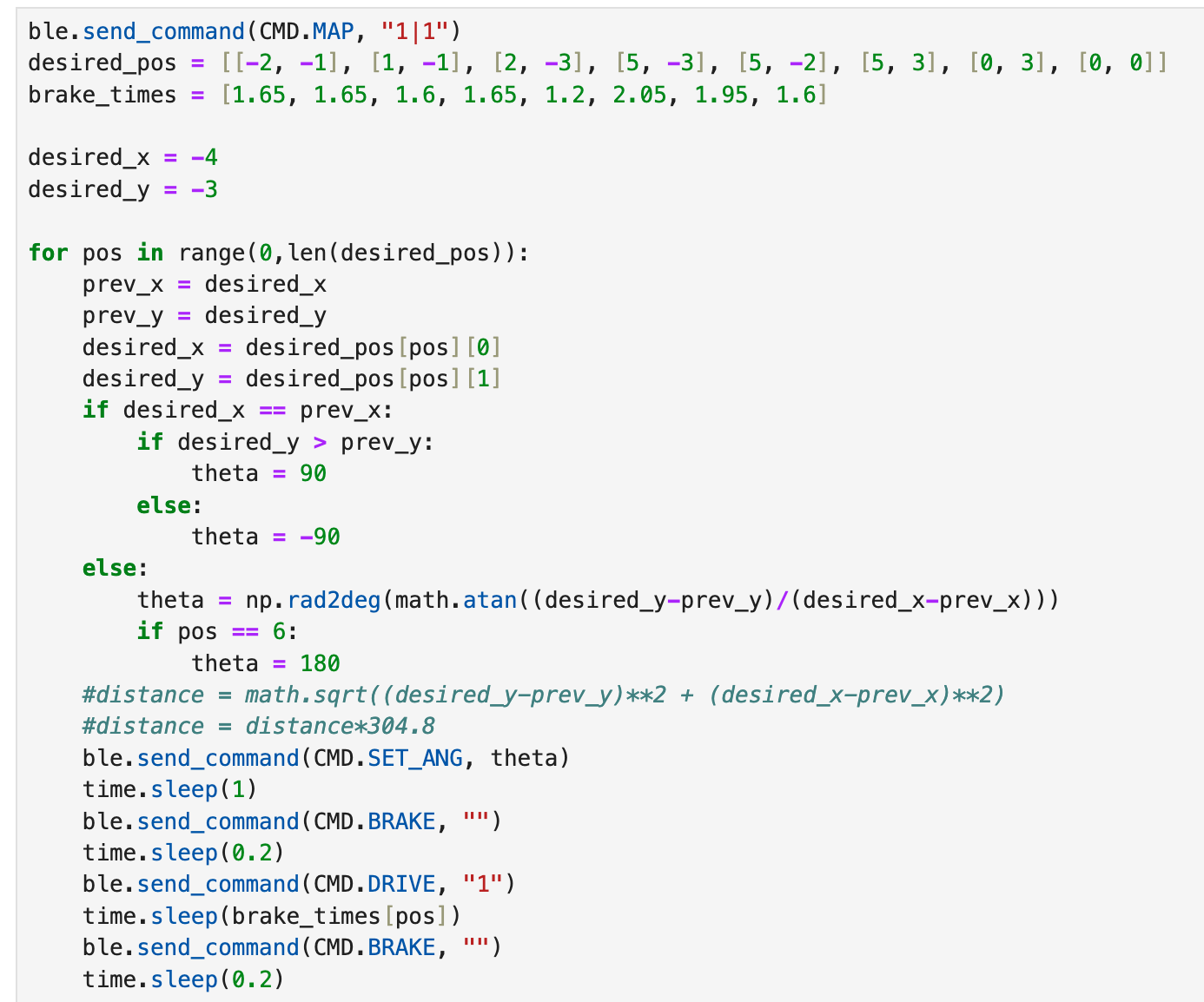
As seen above, even hard coding is not perfect. The primary reason for this is that the gyroscope drifts over time, as described in previous labs. This makes it difficult to reliably turn over and over again, especially when there is a distance between the points and the robot might not drive perfectly straight. A future fix for this issue could be to do continuous orientation control while the robot is moving straight. This would require additional math when it comes to calculating the speed of each wheel, but it would ensure that the robot drives straight and reaches its correct waypoint. Below is my Jupyter code that was the main control behind my trials.

Lab 12 Takeaways
Overall, this was definitely the most challenging lab, and I wish I had more time to spend on the localization or ToF navigation plans. I think it would have been much more rewarding to see my robot successfully navigate using more of an autonomous approach. However, I think I am still proud of the work done in this lab as well as the class as a whole. I struggled a lot but learned even more, and I am definitely walking away with my head held high. I want to thank the TAs for their hard work this semester and all of their help throughout lab hours. Also, thank you Jonathan for a great semester!